Review of Microeconomics
The economic analysis of law makes use of the tools of microeconomics, which, broadly defined, is the study of how individuals make decisions in the presence of scarcity. By scarcity, we mean constraints on an individual�s wealth or income, but also on his or her time, knowledge, or information. An economic theory of decision making assumes that individuals act rationally in the sense that they make decisions that best promote their well-being (however that is defined) given their constraints. Many assume that this approach to decision making is only suited to choices individuals make in a market setting, like what goods to buy or what jobs to take, but economists have applied the tools of microeconomics to a wide range of nonmarket contexts. One of the most successful of these applications has been the economic analysis of law.
Before embarking on this analysis, however, it is essential that students have a firm grasp of the basic tools of microeconomics. The purpose of this appendix is to review those tools. The discussion is necessarily brief and is not meant to be a substitute for a full semester course on the principles of microeconomics. Rather, it is intended as a �brush up� for students who have already had such a course.
We begin with the theory of the consumer, which describes the optimal choices of individual consumers or households. By aggregating across all consumers, we can derive the market demand curve for a particular good or service. We then turn to the supply side, which is based on the study of business firms. Individual firms make production decisions to maximize profits, and by aggregating the output decisions of all firms, we can derive the market supply.
Equilibrium is found by combining the demand and supply sides of the market. The nature of the equilibrium, however, depends on the organization of production on the supply side. If there are many firms, the industry is competitive, but if there is only one, it is monopolistic. We review both of these types of industries, but we pay special attention to the intermediate case where there are a few firms, what economists call oligopolies. Deriving the equilibrium in oligopolistic industries requires the introduction of a powerful tool called game theory, which describes the strategic interaction of a small number of decision makers. The principles of game theory will prove useful in many legal contexts as well.
Following our discussion of market equilibrium, we turn to welfare economics, which concerns the goals of an economic system, both in terms of how efficiently resources are allocated and also how fairly. An important aspect of welfare economics is the study of how externalities lead to market failure and the various remedies that are available to policymakers. We will see that the economic analysis of law is largely about how the law responds to various forms of market failure.
The final section of this appendix is about uncertainty and imperfect information. We will see that much of the law can be understood as a response to imperfect and costly information on the part of decision makers. Thus, understanding how economists incorporate these factors into their models will prove crucial to our analysis throughout this book
1 The Theory of the Consumer and Market Demand
The economic theory of consumer choice is based on the notion of rationality. That is, consumers are assumed to make choices that yield them the highest level of well-being subject to the constraints that they face. Underlying this model of choice is the idea that consumers have well-defined preferences over their array of choices. These preferences are summarized by a utility function that allows consumers to rank the various bundles of goods and services that are available to them.
To keep things simple, suppose that there are only two goods available to a particular consumer, pizza and beer. Let x denote the quantity of pizza that the individual consumes and y the amount of beer. The utility function u = u(x, y) describes the level of well-being, or satisfaction, that the individual gets from any combination of these two goods. The specific value of u has no particular meaning except that higher values of u indicate that the individual has achieved a higher level of satisfaction.
We assume that both pizza and beer are �goods� in the sense that more of each causes utility to rise. Thus, u(2, 1) > u(1, 1) because the individual is happier with two slices of pizza than with one, holding the number of beers fixed at one. Similarly, u(1, 2) > u(1, 1). You might be wondering at this point why we need a utility function at all if we only care about ranking bundles, and more of a good always makes the consumer better off. The reason is that sometimes, the consumer has to compare bundles in which the amount of one good increases while the amount of the other decreases. For example, suppose you are given the choice between these two bundles: (2, 1) and (1, 2). In order to rank them, you need to decide whether you value one more slice of pizza more than one more beer. The utility function, as a reflection of each individual�s preferences, summarizes this choice.
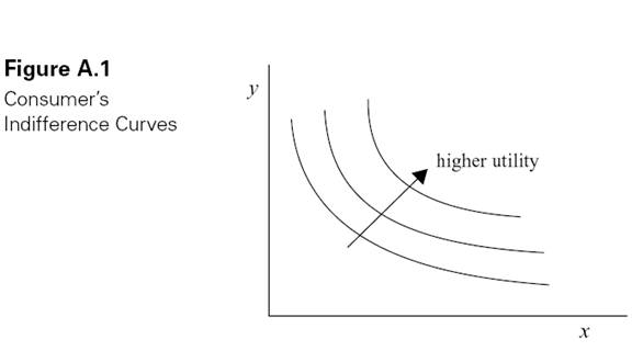
One reason for limiting our model to two goods is because it allows us to provide a graphical representation of the utility function. Figure A.1 shows the �indifference curves� associated with a particular individual�s utility function over the goods x and y. An indifference curve is defined to be all those combinations of x and y that yield the consumer the same level of satisfaction. Movement to a higher indifference curve corresponds to a higher level of satisfaction, and movement to a lower curve to a lower level of satisfaction. Indifference curves thus represent a sort of �topographical map� of the consumer�s preferences.
What prevents individuals from consuming ever higher levels of both goods and thereby achieving higher levels of satisfaction? The answer is that goods cost money and consumers have limited income with which to buy them. The problem for the consumer, therefore, is to choose the bundle of goods that yields the highest level of utility and is also affordable, given income and prices. In order to solve this constrained maximization problem, we first need to find those combinations of x and y that are affordable.
If px and py are the prices of the goods and I is income, then the affordable bundles must satisfy the following budget equation:
pxx + pyy = I.��������������������������������������������������������������������������������������� (A.1)
This equation is graphed in Figure A.2 as a negatively sloped straight line with slope equal to −px/py, vertical intercept at I/py and horizontal intercept at I/px.1 All points on this line cost exactly I dollars, while points above it cost more than I and points below it cost less than I.
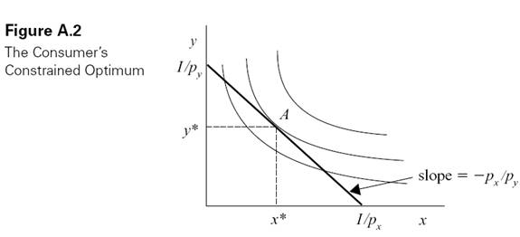
The consumer�s optimal point is found by locating the highest indifference that just touches the budget line. This point, indicated by point A in Figure A.2, is therefore the combination of x and y that yields the highest level of utility while just exhausting the consumer�s income. The resulting consumption bundle is denoted (x*, y*).
Note that at this optimal point, the slope of the indifference curve, or the marginal rate of substitution, equals the slope of the budget line, which we saw above is equal to the absolute value of the price ratio. Thus, at the optimal point, the rate at which the consumer is willing to exchange one good for the other in order to maintain the same level of well-being (or utility) exactly equals the rate at which he can exchange them while keeping the same level of expenditure.
Point A in Figure A.2 shows the consumer�s optimal choice of goods x and y, holding prices and income fixed. If income or prices change, however, the consumer�s optimal bundle will change. For example, suppose that the price of good x decreases, holding py and I fixed. The effect on the budget line in Figure A.2 is that the vertical intercept remains fixed at I/py, while the slope flattens and the horizontal intercept shifts out. In other words, the budget line rotates outward around the fixed vertical intercept. The new optimum therefore occurs on a higher indifference curve with the consumer consuming more of the cheaper good x. However, the impact on good y, whose price has not changed, is ambiguous.
By repeating this process for different values of px, we can derive the individual demand curve for good x, which is defined to be the optimal quantity of x demanded by this consumer for any price, holding his or her income and the prices of all other goods fixed. Then, by adding up the quantity demanded by all consumers at each value of px, we can derive the aggregate, or market demand curve for good x. This is shown in Figure A.3. The negative slope reflects the Law of Demand, which says that the quantity demanded of a good falls as its price increases.
The demand for good x also varies with consumers� income and the price of y. We can see how by returning to the individual consumer�s optimum.
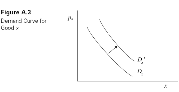
Note that, beginning from the initial point A, if income increases holding px and py fixed, the budget line shifts out parallel. As a result, the consumers will be able to achieve a higher indifference curve and will (probably) purchase more of both x and y.2 The individual demand curves for good x will therefore shift out, causing the aggregate demand curve to shift out as well, as shown by the curve labeled Dx′ in Figure A.3. The outward shift means that for any px, consumers demand more of good x as their incomes rise.
The demand for x is also a function of the prices of other goods. Suppose, for example, that the price of y increases, holding px and I fixed. The budget line in Figure A.2 therefore rotates downward around the fixed horizontal intercept, I/px, resulting in a tangency on a lower indifference curve. The consumer will demand less of good y, but he may consume more or less of good x. Thus, in aggregate, the demand for good x may rise or fall with an increase in the price of good y. If it rises (causing the demand curve to shift out), we say that x and y are substitutes; if it falls (causing the demand curve to shift in), we say that x and y are complements.
An important characteristic of demand curves is how responsive demand is to changes in price. Economists measure this responsiveness by calculating the elasticity of demand, which is defined to be the percentage change in quantity demanded in response to a 1 percent change in price.3 The formula for elasticity of x with respect to changes in px is
�����������  ���(A.2)
where Δx is the change in quantity of x demanded, and Δpx is the change in price.4 For example, suppose that the price of gasoline rises from $1.00 to $1.10 per gallon, causing the daily demand for gas at a particular station to fall from 500 to 475 gallons. The elasticity of demand over this range of the demand curve is therefore given by5
�����������  (A.3)
(A.3)
Note that the elasticity is a negative number because quantity and price move in opposite directions along the demand curve (reflecting its negative slope). Since people usually find it easier to work with positive numbers, however, elasticity is often reported as an absolute value. Thus, we would say that the elasticity of demand in the above example is .5, which means that a 1 percent increase in the price of gas results in a .5 percent decrease in the demand for gas.
The fact that the elasticity in this example is less than one (in absolute value) means that the demand is relatively inelastic. In other words, quantity changes more slowly than price in percentage terms. In contrast, if elasticity is greater than one, quantity changes faster than price in percentage terms. In this case, we say that demand is relatively elastic. When price and quantity change at the same rate, we say that demand has unitary elasticity because ε = 1. It should be clear that information about demand elasticity is important because, for example, it allows businesses to predict the impact of price changes on the demand for their product and policymakers to project the revenue that will be generated by a tax that causes the price of a good to rise.
2 The Theory of the Firm and Market Supply
The supply side of the market is based on the decisions of individual business firms whose goal is to maximize profits. The primary activity of firms is production, which involves the transformation of various inputs into outputs that are then sold to consumers as finished goods or to other firms as intermediate inputs. The process underlying production is technological rather than economic in nature, and thus economists take it as given in the same way that they take consumer preferences as given.
Mathematically, the firm�s production technology is described by the production function, which specifies the way inputs are transformed into output. For example, suppose that a firm combines two inputs, capital, K, and labor, L, into output according to the functional relationship
Q = f(K, L),���������������������������������������������������������������������������������������������������� (A.4)
where Q is the quantity of output produced. The problem for the firm is to choose the quantities of the two inputs to maximize profit, which is equal to the total revenue from sale of the output less the costs of the two inputs. This problem is usually broken into two parts: the firm first chooses the combination of inputs that minimizes total costs for each level of output, and then chooses output to maximize revenue minus costs. We consider these problems in turn.
The firm�s total input costs are given by the cost equation
C = pKK + pLL,����������������������������������������������������������������������������������������������� (A.5)
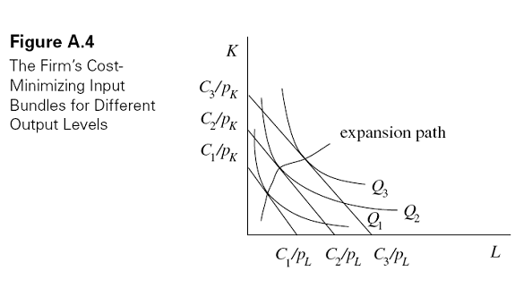
where pK and pL are the input prices, which the firm takes as given. Note that this equation resembles the consumer�s budget constraint, and it can be graphed in much the same way. This is shown in Figure A.4, which graphs three cost lines corresponding to three levels of total costs. Along each line, total costs are the same, but costs increase as we move to higher lines because the firm is using more inputs. Thus, C3 > C2 > C1.
As noted, the firm chooses the input combination that minimizes costs for each possible level of output. To solve this problem, we first need to represent the production function graphically. It turns out that we can do this in the same way that we graphed the consumer�s utility function. That is, we find all those combinations of K and L that yield a given level of output and connect them to form a line called an isoquant (meaning �same quantity�). A set of three isoquants is shown in Figure A.4, corresponding to three output levels, Q1, Q2, and Q3. Note that isoquants look like indifference curves, and like utility, output is increasing as we move up and to the right, implying that Q3 > Q2 > Q1. Just as more consumption goods yield consumers more utility, more inputs allow the firm to produce more output.
The tangency points of each isoquant with a cost line show the optimal input combinations for the particular output level. This is true because, for each isoquant, the tangency point represents the lowest cost line that allows the firm to produce that level of output. The set of all tangency points, represented by the expansion path in Figure A.4, thus shows the cost-minimizing combination of inputs for all possible output levels. Note that the expansion path defines a relationship between total costs (C) and output (Q), which we call the firm�s total cost function, written as C(Q).
Associated with the total cost function is the marginal cost function, which is defined to be the increment in total costs when output is increased by one unit. Mathematically, it is given by the slope of the total cost function, or
���������� ��������������������������������������������������������������������������������������������������� (A.6)
This quantity will be crucial for determining the firm�s profit-maximizing output level. We can also define the firm�s average cost to be the ratio of total cost to output, or
����������� ��������������������������������������������������������������������������������������������������� (A.7)
We are now in a position to derive the firm�s profit-maximizing level of output. Here, we consider a competitive firm that takes the output price, P, as given. Below, we consider alternative market structures. The profit expression for a competitive firm is given by
Π = PQ − C(Q),���������������������������������������������������������������������������������������������� (A.8)
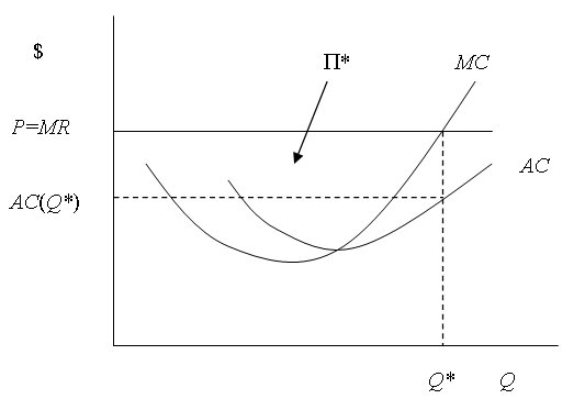
where PQ is total revenue. To maximize profits, the firm increases output to the point where the revenue from the last unit sold (marginal revenue) equals the cost of producing the last unit (marginal cost). Since the price is constant for a competitive firm, marginal revenue equals price, and the profit-maximizing output occurs at the point where
P = MC.��������������������������������������������������������������������������������������������������������� (A.9)
This condition is shown graphically in Figure A.5. Note that marginal cost is drawn as a U-shaped curve, meaning that marginal costs first fall but eventually rise as output increases. This reflects the underlying technology of the firm and suggests that firms cannot expand indefinitely without eventually experiencing an increase in the cost of producing additional units. Because of its shape, marginal cost intersects price at two points. Profits are maximized at the point where marginal costs are rising, yielding optimal output of Q*.6
Figure A.5 also shows the average cost curve of the firm.7 Note that at the profit-maximizing output level, price is above average cost. Thus, the firm is earning a positive profit in the amount
Π* = (P − AC(Q*))Q*.����������������������������������������������������������������������������������� (A.10)
Graphically, this amount is shown by the rectangle labeled Π*. Since the firm is earning a positive profit, the equilibrium shown in Figure A.5 must be a short-run equilibrium. In economics, the short run is defined to be the period of time during which the firm holds one or more inputs fixed, and new firms are not able to enter the industry. In the long run, all inputs become variable and new firms can enter, assuming that no barriers to entry exist. New firms are attracted to an industry if existing firms are earning positive profits. As entry occurs, output of the good increases and the market price falls. At the same time, greater competition for inputs causes firms� costs to rise. The combination of these factors reduces the profit of all firms in the industry until they are driven to zero, at which point entry into the industry ceases. At this point, we are in a long-run equilibrium in which all firms earn zero profits.
Figure A.5 The Competitive Firm�s Profit-Maximizing Output |
 |
Let us now turn from the individual firm to the industry in order to derive the industry supply curve. The supply curve shows the aggregate quantity of a good that firms will supply to the market at a given price. For each individual firm, we have seen that the amount it will supply at any price is found by moving along the upward-sloping portion of its marginal cost curve since P = MC defines its profit-maximizing output. Thus, as was true in the case of demand, if we horizontally add all the firm marginal cost curves we will obtain the market supply curve.8 The upward slope of the supply curve therefore reflects the increasing marginal costs of firms.
Now that we have derived the market demand and supply curves, we can show how they interact to yield the equilibrium quantity and price.
3 Market Equilibrium
The nature of the market equilibrium depends on the organization of the industry producing the good in question. In deriving the supply curve in the previous section, we assumed that the industry was competitive. We therefore begin by examining the equilibrium of a competitive industry. Later, we consider alternative market structures.
��������� 3.1���� Perfect Competition
The defining characteristic of a competitive industry is that there is a large enough number of suppliers that no one supplier believes that its output decision will affect the price. This is why we assumed above that individual firms take the price as given. In fact, the price is determined in equilibrium, along with output, by the intersection of the supply and demand curves as shown in Figure A.6. At this intersection point, the amount of the good that consumers want to buy at the set price exactly equals the amount that producers supply to the market. In other words, there is no incentive for either buyers or sellers to change their behavior. This is the sense in which the price and quantity pair (Pe, Qe) constitute an equilibrium.
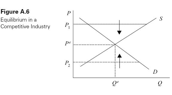
Further, if the market ever deviates from this equilibrium point, there are forces that will tend to drive it back there. Suppose, for example, that the price is above Pe, say at P1 in Figure A.6. At this price, the amount producers want to supply to the market exceeds the amount that consumers want to buy. We say there is excess supply, which manifests itself in a growing inventory on store shelves. Firms respond by lowering their prices until the excess supply is eliminated.
Alternatively, suppose price is below Pe, say at P2. At this price, consumers demand more of the good than sellers are willing to provide. We say there is excess demand, which results in waiting lines and backorders. Firms respond by raising their prices until the excess demand is eliminated. In either case, equilibrium is reestablished by the actions of individual buyers and sellers acting in their own self-interest.
����������� Example: The Algebra of Supply and Demand.
The equilibrium output and price in Figure A.6 can also be derived algebraically. This is especially easy in the case of straight-line supply and demand curves. Let the equations for supply and demand be given by
����������� Ps = a + bQ
����������� Pd = c - dQ
where c > a (so that the demand curve has a higher intercept than the supply curve), and b and d are positive. Together, these assumptions ensure that supply and demand intersect in the positive quadrant. To find the equilibrium, set Ps = Pd and solve for Q to obtain
����������� 
which is positive given c > a. Now substitute Qe into either the supply or demand equation to get
����������� 
As an example, let a = 10, c = 50, and b = d = 1. Then we have Qe = 20 and Pe = $30.
��������� 3.2���� Monopoly
At the opposite extreme from perfect competition is monopoly, which occurs when a single seller serves the entire market. A monopoly can arise for several reasons, but the two most important reasons are technological and legal. The technological reason for monopoly is the existence of significant economies of scale in production, which means that average costs are falling over the relevant range of production. In this case, it is actually efficient to create a monopoly because if production were divided up into multiple firms, average costs would rise. A market that is efficiently organized as a monopoly for this reason is called a natural monopoly.
The problem with natural monopoly is that a single private firm will set the monopoly price and output levels, which are inefficient. Thus, natural monopolies are generally either regulated (like utilities), or operated as public enterprises.
The legal reason for monopoly is the issuance of a patent by the government to a firm that invents a new product or production process. A patent is an exclusive and legally enforceable right to benefit from the invention. As Chapter 6 shows, the economic reason for granting of patents is to encourage invention by allowing innovators to appropriate the returns from their efforts. This must be balanced, however, against the social loss from creation of a monopoly. Thus, the life of a patent is limited to a fixed number of years, after which competing firms are allowed to enter the industry and profit from the invention.
Monopolistic firms seek to maximize profit, just like competitive firms, but their output and pricing decisions are different, which accounts for the inefficiency of monopoly. The monopolist, like the competitor, produces output at the point where marginal revenue equals marginal cost. Marginal cost is the same as for a competitive firm, but marginal revenue differs.9 Recall that marginal revenue is defined to be the additional revenue from selling one more unit of output. For a competitive firm that takes price as given, MR = P, but for a monopolist, marginal revenue is less than the price. The reason is that the monopolist faces the market demand curve, which is downward sloping. Thus, in order to sell an additional unit of the good, it must lower the price for that unit, as well as for all previous units. (This assumes that all customers are charged the same price for the good; that is, the monopolist does not practice price discrimination.)
To illustrate, suppose the monopolist can sell 10 units of a good for $50, yielding total revenue of $500. In order to sell 11 units, however, it must lower the price to $48, which yields total revenue of $528. The marginal revenue is thus $28, which is less than the price. Marginal revenue is actually made up of two components: the gain of $48 from selling the 11th unit, less the loss of $20 from selling each of the first ten units for $2 less. Together, these amounts yield the net gain of $28. It should be clear from this example that marginal revenue will be negative if the loss in revenue from lowering the price exceeds the gain from selling the additional unit. The monopolist, however, will always produce in the range where MR > 0. (This is true because at the optimum, MR = MC.)
Figure A.7 The Monopolist�s Optimal Output and Price Level |
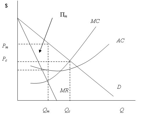 |
Figure A.7 graphs the demand and marginal revenue curves facing a monopolist, along with the monopolist�s marginal and average cost curves. The profit-maximizing output, denoted Qm, occurs at the intersection of the MR and MC curves. For comparison, the graph shows the output that would be produced if the industry were competitive, Qc, which occurs at the intersection of the MC and D curves. Since marginal revenue is always less than price for a downward-sloping demand curve, monopoly output will always be less than the corresponding competitive output.
The price charged by the monopolist, Pm, is found by locating the point on the demand curve corresponding to optimal output. This represents the highest amount consumers are willing to pay for that level of output. The monopoly price is clearly higher than the price that would prevail in a competitive industry, which is given by Pc. Finally the monopolist�s profit is shown by the rectangle labeled Πm, which is the area between price and average cost over the range of production.
The inefficiency associated with monopoly is due to underproduction relative to a competitive industry. The reason for the inefficiency is that the demand curve exceeds the firm�s marginal cost curve over the range of underproduction (the range between Qm and Qc in Figure A.7). Thus, by failing to produce those units, the economy foregoes the surplus represented by the difference between what consumers are willing to pay for the good and what it costs to produce it. This foregone surplus is referred to as the deadweight loss from monopoly. This loss is one reason for government regulation of monopoly, as detailed in Chapter 10.
��������� 3.3���� Oligopoly and Game Theory
Intermediate between perfect competition and monopoly is oligopoly, which occurs when a few firms serve an industry. This is perhaps a more realistic market structure than either competition or monopoly, but it is also more difficult to analyze because firms must account for the interdependence of their output and pricing decisions. The key to analyzing oligopolistic markets is therefore the assumptions firms make about the behavior of their rivals.
Economists have developed several models of oligopoly, some of which are more realistic than others. Probably the best of these models is based on the economic theory of games (or game theory), which provides a general theory of strategic interaction between economic agents. It is therefore ideally suited to describing the behavior of a few competing firms. Since game theory has many applications in the economic analysis of law, we provide a brief overview here with an application to oligopoly.
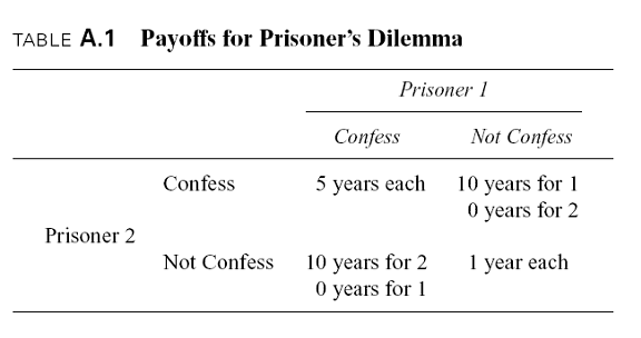
The best way to describe game theory is in the context of a specific example. Probably the most famous game, and one closely related to the problem facing oligopolists, is the prisoner�s dilemma.10 In this game, two suspects are apprehended for a serious crime that carries a prison term of ten years, but the prosecutor only has evidence sufficient to convict them of a lesser offense carrying a sentence of one year. Each prisoner is therefore offered a deal: if he confesses and testifies against the other, he will be released, provided that the other prisoner remains silent. However, if both confess, they will be convicted of the serious crime and receive reduced sentences of five years each.
Each prisoner therefore chooses between two strategies: confess or not confess. Table A.1 shows the sentence for each prisoner as function of their strategies. In making their choices, the prisoners are assumed to minimize their sentence, and they are not allowed to communicate with each other.
Consider first the behavior of prisoner 1. Since he does not know which strategy prisoner 2 will employ, he derives his optimal choice for each of prisoner 2�s options. First, if prisoner 2 confesses, it is best for prisoner 1 to confess as well since he receives five rather than ten years. Alternatively, if prisoner 2 chooses not to confess, it is again best for prisoner 1 to confess since he gets no prison term rather than 1 year. Since prisoner 1 is better off confessing regardless of prisoner 2�s choice, we say that confessing is a dominant strategy for prisoner 1. It should be clear that the same logic applies to the optimal strategy of prisoner 2, which means that the equilibrium of this game is for both prisoners to confess. This outcome is an equilibrium because neither party wishes to change his behavior given the behavior of the other player. Such an equilibrium is referred to as a Nash equilibrium.
It is interesting to note that the Nash equilibrium of the prisoner�s dilemma does not minimize the combined prison sentences of the two players. In particular, if both had chosen not to confess, they would have received one year each rather than five each. It will often be the case that the equilibrium of a game is different from the optimal outcome, which is the outcome that the players would have chosen if they were able to make binding commitments to each other. This aspect of the prisoner�s dilemma proves useful in understanding why it is so difficult for oligopolistic firms to sustain a collusive (or cartel) outcome.
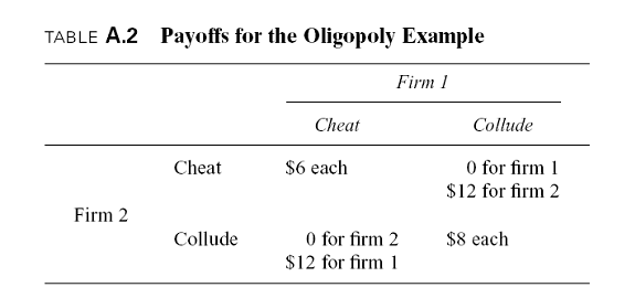
In order to translate the prisoner�s dilemma into the oligopoly case, consider two rival firms who share a particular market. In order to maximize their joint profit, they would collude and set the monopoly output and price. Suppose this would yield each of them $8 in profit. However, if either firm deviates from this outcome by lowering its price slightly while the other firm abides by the agreement, the cheating firm will capture the entire market, yielding a profit of, say, $12. However, if both firms cheat, they will again share the market, yielding profit of $6 each. Table A.2 summarizes the payoffs to the two firms as a function of their strategies.
It should be easy to see that this game has the same structure as the prisoner�s dilemma (except that the players wish to maximize profit rather than to minimize their sentences). Thus, the dominant strategy for both firms is to cheat, which yields them less profit than if they had been able to sustain the collusive agreement. This example shows why it is so difficult for cartels like OPEC to keep their prices high.
Many economically interesting games do not have dominant strategies, but they always have Nash equilibria. Thus, we conclude our brief discussion of game theory by deriving the Nash equilibrium of a game that does not have dominant strategies. Consider, for example, the coordination game shown in Table A.3.11 There are two players, labeled 1 and 2, each of whom can choose to play either �left� or �right.� If both choose the same strategy (regardless of which one), they each receive a payoff of 1, but if they choose opposite strategies, they each receive zero. An example is the choice of two motorists, traveling in opposite directions on the same road, regarding which side of the road to drive on.
To find the Nash equilibrium of this game, consider first player 1�s optimal strategy given each of player 2�s choices. If 2 is expected to play left, it is best for 1 to play left, but if 2 is expected to play right, it is best for 1 to play right. The reasoning is symmetric regarding player 2�s optimal strategy. Clearly, there are no dominant strategies as in the prisoner�s dilemma game, but there are two Nash equilibria.12 One occurs when both choose left, and the other occurs when both choose right. In each case, neither player wants to alter his strategy given the choice of the other. The problem is that there is nothing in the game itself that tells us which of these equilibria is likely to arise. Thus, there is a real possibility of a �coordination failure.�
One way to avoid coordination failure is for the players to communicate with each other before or during the game. Another is for the law to force one of the equilibria to occur.
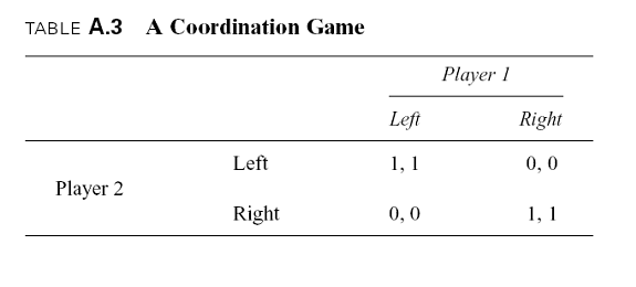
In the game in Table A.3, it doesn�t matter which one the law chooses since the payoffs are the same. Thus, for example, there is no inherent advantage of a law requiring all motorists to drive on the right over one requiring them to drive on the left, so long as one is enacted.
4 Welfare Economics
Welfare economics is that area of economics concerned with evaluating the performance of the economy regarding its impact on the well-being of consumers. In this context, we consider both how efficiently the market allocates resources, and how fairly it distributes income. Failure of the market along either of these dimensions (efficiency or fairness) provides a possible basis for government intervention.
��������� 4.1���� Welfare Theorems
One of the most important results in economic theory concerns the ability of the market mechanism to coordinate the behavior of individual consumers and firms so as to achieve an efficient allocation of resources. As far back as 1776, Adam Smith recognized the power of competitive markets to do this without conscious direction, as if by an �invisible hand.� Modern microeconomics has established this conclusion more rigorously in the form of the First Fundamental Theorem of Welfare Economics, which is sometimes referred to as the Invisible Hand Theorem in tribute to Smith�s early statement of this result.
The Invisible Hand Theorem says that competitive markets will be efficient in the sense that no reallocation of resources can increase the size of the social pie, but it says nothing about how the pie is divided. In fact, the final distribution of wealth depends crucially on the initial endowments of resources. If that distribution was unequal to begin with, it will likely remain unequal in a competitive equilibrium. This suggests that efficiency and fairness may be in conflict with one another. Fortunately, there is another important result in welfare economics, called the Second Fundamental Theorem, which says that any distribution of wealth can be achieved by a competitive equilibrium provided that lump sum transfers of wealth are possible. Thus, under certain conditions, efficiency and fairness are not incompatible. (Chapters 1 and 6 show that in this respect the Second Fundamental Theorem is closely related to the Coase Theorem.) Unfortunately, realistic methods for redistributing income, such as income and wealth taxes, create distortions in the market that lead to inefficiency. Practically speaking, therefore, policymakers do generally face a trade-off between fairness and efficiency.
��������� 4.2���� Market Failure
The efficiency of markets requires that the conditions of perfect competition prevail. When one or more of these conditions are not met, we have a case of market failure. We have already encountered one reason for market failure: monopoly. As shown above, monopoly causes inefficiency because the monopolist underproduces the good in question, thus depriving the economy of the gains from trade over the range of underproduction. As noted, this logic is the basis for laws aimed at preventing, or in the case of natural monopoly, regulating, the exercise of monopoly power.
A second source of market failure is the existence of externalities. An externality exists when an individual or firm imposes a benefit or cost on some other individual who either does not have to pay for the benefit, or is not compensated for the cost. The most common example of an external cost (or negative externality) is pollution. When a firm�s production process requires it to emit smoke or other waste that is harmful to others, the firm is in effect using the victims� good health as an input in production but is not required to pay for that input. Since people value their health, the firm is therefore overusing this input and, as a result, is overproducing the good in question.
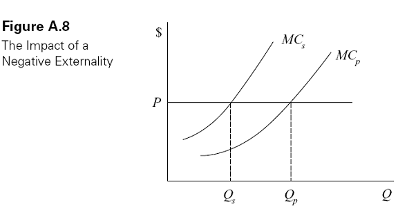
Another way to say this is that the firm�s private marginal cost, which reflects the costs of the inputs that it actually has to pay for, is less than the social marginal cost, which reflects the true cost of the inputs to society, including any harm to pollution victims. This characterization of a negative externality is shown in Figure A.8, where MCp is the private marginal cost and MCs is the social marginal cost. The vertical distance between the curves is the amount of the external cost. A profit-maximizing, competitive firm will produce at the point where price equals MCp (the point labeled Qp), rather than at the socially optimal point, Qs, where price equals MCs. In contrast to monopoly, which results in inefficiency due to underproduction, a negative externality causes inefficiency due to overproduction.
Economists commonly propose the use of taxes as a way to eliminate the inefficiency due to negative externalities. The purpose of the tax is to force the firm to internalize the cost of harm it imposes on victims of pollution. In Figure A.8, a pollution tax (often referred to as a Pigovian tax after the economist Arthur Pigou) would have the effect of shifting up the private marginal cost curve until it intersects price at the socially optimal output level.� Much of the economic analysis of law is concerned with internalizing externalities.�
����������� A third source of market failure is the existence of public goods. A pure public good is characterized by two properties. First, it is inexhaustible, which means that consumption of the good by one person does not reduce the quantity available for others. For example, a radio broadcast is inexhaustible because, once the signal is transmitted, any number of people can turn on their radios without reducing the quality of the program for others. In contrast, an apple is exhaustible�and hence a private good�because once you eat it, it cannot be consumed by others. The second characteristic of a public good is that it is nonexclusive, which means that once the good is produced, no one can be denied consumption, even if they have not paid for it. Again, a radio broadcast is a good example. The ability of nonpayers to consume a public good is referred to as the free-rider problem.
The inefficiency created by public goods is that private firms will generally be unwilling to provide them (or will underprovide them) because of the free-rider problem. (The financing problems facing public radio and television stations illustrate the difficulty.) For this reason, the government is usually charged with providing (or subsidizing) public goods because it can use its tax power to coerce people to contribute to their provision.
5 Uncertainty and Imperfect Information
In addition to the above sources of market failure, lack of perfect information can lead to inefficiency. Problems of imperfect information will arise throughout the law, so it is essential for students to have a basic understanding of how economists incorporate information into their models. We begin by examining choice under uncertainty and the economic theory of insurance.
��������� 5.1���� Choice Under Uncertainty and Insurance
Most choices we make involve some amount of uncertainty about the possible consequences. Consider, for example, the act of driving a car. Every time a person gets into a car there is a risk of an accident, so why do people do it? Obviously, the gains from driving exceed the cost. The way economists show this is by calculating the expected value of driving.
 �
�
Suppose that the costs and benefits of driving can all be expressed in monetary terms. Specifically, suppose that the gain from driving is $500 per month, but there is a one in one hundred chance of an accident involving a loss of $10,000. The expected value of driving is thus
EV = (.99)($500) + (.01)($500 − $10,000) = $500 − (.01)($10,000) = $400. (A.11)
Driving therefore yields an expected gain of $400. In general, the expected value of any action involving uncertain outcomes is equal to the sum of all possible outcomes weighted by their probabilities.
Our analysis of consumer choice above showed that people make decisions based on utility, not income. Thus, they calculate the expected utility of driving rather than the expected income. This is easily done as follows. Let U(I) be an individual�s utility over income, and suppose her monthly income is Y if she never drives. Thus, if she drives, her utility is U(Y + $500) if no accident occurs, and U(Y + $500 − $10,000) if one does occur. Her expected utility is the sum of these utilities weighted by their probabilities:
EU = (.99)U(Y + $500) + (.01)U(Y − $9,500).����������������������������������������������� (A.12)
The individual will choose to drive if this expression exceeds the utility from not driving, which is a certain value equal to U(Y).
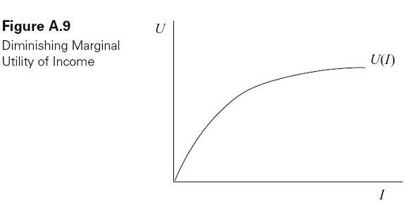
Economists usually assume that people�s preferences are characterized by diminishing marginal utility of income. Intuitively, this simply means that as people become richer, they value an additional dollar less. Formally, it means that the slope of the utility function flattens as income goes up. In other words, the utility function is concave in income, as shown in Figure A.9.
What evidence do we have that people actually have preferences of this sort? One important piece of evidence is that they routinely buy insurance. We will see that a person who has diminishing marginal utility of income is also risk averse in the sense that she will pay some amount of money in order to avoid risk. The fact that people will pay to avoid risk is what makes it possible for insurance companies to make a profit.
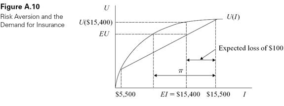
The maximum amount of money a risk-averse person will pay for insurance against a car accident is shown in Figure A.10. Suppose that Y = $15,000 in the above example, so that the driver�s income in the no-accident state is $15,500, but her income in the accident state is $5,500. Her expected income is therefore
EI = (.99)($15,500) + (.01)($5,500) = $15,400.
At the same time, her expected utility is
EU = (.99)U($15,500) + (.01)U($5,500).
As shown in the graph, the fact that the driver has diminishing marginal utility of income implies that she is better off with a certain income of $15,400 than with an uncertain income that has the same expected monetary value. That is
U($15,400) > EU.������������������������������������������������������������������������������������������ (A.13)
It follows that the driver will be willing to pay some amount of money to avoid the risk associated with accidents. Specifically, she will pay up to π as an insurance premium, where U($15,500 − π) = EU as shown in Figure A.10.
The function of insurance in this setting is to convert an uncertain income for the driver into a certain income by promising full compensation for her losses in the event of an accident in return for a fixed premium. The insurance company, which is assumed to be risk neutral (that is, it cares only about expected income), is able to make a profit from the policy because the premium, π, exceeds the expected loss of (.01)($10,000) = $100. This is also shown in Figure A.10.
5.2 Moral Hazard
The preceding analysis treated the probability of an accident as fixed, but in reality, drivers make choices that affect this probability, such as how fast to drive and how well to maintain their car. Since these precautions are costly, however, insured drivers will tend to underinvest in them from a social perspective because they do not internalize the full benefits of reducing the probability of an accident. This problem, which economists refer to as moral hazard, tends to increase the cost of insurance.
One way insurance companies deal with moral hazard is by offering policies with �deductibles,� or provisions that require consumers to pay the first, say, $500 of any accident claim. By holding consumers responsible for some of the costs of an accident, deductibles increase incentives for precaution and discourage the filing of small claims. Thus, policies with higher deductibles have lower premiums.
Moral hazard problems are not limited to insurance contexts, however. They also arise in rental arrangements where the ownership and use of a durable asset, like a house, car, or farmland, are divided. Since users have no claim on the residual value of the asset, they have an incentive to overutilize or undermaintain it. Thus, rental contracts typically include provisions like security deposits aimed at mitigating this problem.
Another area where moral hazard occurs is in employment relationships where worker effort affects output but is unobservable to the employer. In this setting, if workers are paid a fixed wage or salary, they have little incentive to work hard. Thus, many employment contracts condition an employee�s compensation, at least partially, on some measure of output, as when a salesperson is paid a base wage plus a commission.
As an example, consider the following general compensation scheme
w = a + bQ,���������������������������������������������������������������������������������������������������� (A.14)
where a is a base wage, b is the commission rate (0 ≤ b ≤ 1), and Q is output, which is a function of the worker�s effort and random factors. How are the parameters a and b chosen? One scheme that eliminates the moral hazard problem sets b = 1 and a < 0. That is, the worker makes a fixed payment to the employer and then retains the entire output. In effect, the worker �buys� the business from the owner. An example is a franchise agreement. Under this scheme, the worker exerts optimal effort because she internalizes the full costs and benefits of her actions, but she also bears the full risk of random fluctuations in output (that is, fluctuations unrelated to her effort). Thus, although this scheme is efficient in terms of incentives, risk-averse workers will not find it attractive. They would prefer instead a fixed wage that fully insures them against income fluctuations and imposes the risk on the employer (who is presumably risk neutral). Such a scheme would have a > 0 and b = 0. But this scheme obviously eliminates the incentive for worker effort, as noted above.
What this discussion shows is that there is often a trade-off between optimal risk sharing and incentives (Holmstrom 1979). Thus, the optimal compensation scheme in (A.13) generally balances these two objectives by combining a fixed payment to the worker (a > 0) and a commission rate (0 < b < 1).
��������� 5.3���� Adverse Selection
In addition to unobservable effort, imperfect information in exchange relationships can take the form of unobservable characteristics, such as the quality of a good, the ability of a worker, or the fidelity of a potential spouse. To illustrate the impact of this sort of uncertainty on market outcomes, consider the market for used cars (Akerlof 1970). Assume that used cars are of varying quality known to owners but unobservable to potential buyers. (That is, there is asymmetric information.) Thus, the price for used cars will reflect the average, or expected quality of cars in the market. The problem is that this may cause owners of high-quality used cars to withhold them from the market because they are underpriced. As a result, cars actually available will tend to be from the low end of the quality scale. That is, most will be �lemons.� Economists refer to this as an adverse selection problem.
Market participants respond to adverse selection in several ways. One somewhat controversial response by uninformed parties is statistical discrimination. This is the practice of treating individuals according to the average characteristics of an identifiable group to which they belong. It is commonly used by insurance companies, for example, when they set higher rates for males under age twenty-five as compared to other drivers. Obviously, not all males under twenty-five years old are unsafe drivers, but insurance companies cannot observe the characteristics of individual drivers; they only know that on average, males under twenty-five get into more accidents than other drivers. It may seem unfair to treat drivers differently in this way, but if the insurance company were forced to abandon the practice, rates for drivers outside of the high-risk group would have to be raised, which might push some safe drivers out of the insurance market, creating adverse selection. Given imperfect information, statistical discrimination is therefore a rational practice that improves market efficiency.
Another way insurance companies deal with imperfect information about risk is to offer a menu of contracts that are structured to induce members of different risk groups to �self-select� different contracts. For example, lower-risk drivers might choose policies with higher deductibles and lower premiums because they are less likely to be in an accident (Rothschild and Stiglitz 1976).
A final response to imperfect information involves actions by parties possessing the private information. If a male driver under twenty-five is in fact a safe driver, he would like to �signal� this information to the insurance company so that he can receive a lower rate (Spence 1973). One way he might do this is by maintaining a safe-driving record or getting good grades in school, factors that the insurance company knows are correlated with safe driving and are hard to mimic by unsafe drivers. Another example of signaling is when the manufacturer of a product of unobservable quality offers a warranty covering the cost of defects. Since it is costly for manufacturers to honor warranties, more complete coverage can serve as a signal to consumers that the good in question is of high quality.
Notes
1. To see this, solve (A.1) for y to obtain the equation of a line: y=-(px/py)x+I/py.
2. This assumes that both goods are �normal goods,� which means that their demand increases with income.� If a good is �inferior,� its demand decreases with income, which would cause the demand curve to shift down rather than up.� In the case of two goods, at most one can be inferior since total expenditure must rise with income.
3. Another measure of responsiveness is the slope of the demand curve.� The problem with using slope in this way, however, is that it is sensitive to the units of measure.� Since elasticity measures percentage changes, it is independent of the units of measure.
4. One can also calculate the elasticity of x with respect to the price of y, called the cross-elasticity of demand.
5. The elasticity will generally vary along the demand curve.
6. Condition (A.9) thus represents a �necessary� condition for a maximum.� The requirement that marginal costs be increasing is a �sufficient� condition.
7. Note that the marginal cost curve intersects the average cost curve at the minimum point of the AC curve.� This will be true of any pair of marginal and average cost curves.
8. This procedure will give the short-run supply curve since the number of firms is fixed.� In the long run, the supply curve must account for the entry of new firms as the price rises.
9. We assume that the monopolist�s marginal cost curve is upward sloping and above average costs over the relevant range of production.� As noted, this would not be true for a natural monopolist, whose average costs are falling.
10. See Poundstone (1992) for an interesting history of the prisoner�s dilemma game.
11. See Schelling (1960) for a classic analysis of coordination games.
12. We restrict attention to pure strategies.
